How to Switch Rows and Columns in Excel? Swap

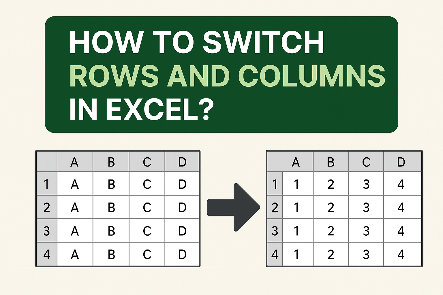
Working with data in Excel often means arranging it in the right way so it’s easy to read and understand. Sometimes you may want to switch rows into columns or columns into rows—for example, turning a vertical list into a horizontal one. This process is called a swap (or transpose), and the good news is it’s very simple to do in Excel. In this blog, we’ll explain step by step how to switch rows and columns in Excel, using easy language so you can organize your data exactly the way you want.

---

Step-by-Step Methods to Swap Rows and Columns

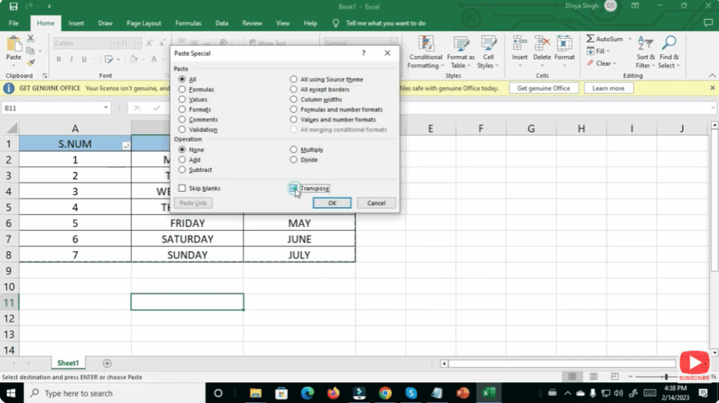
Method 1: Using the Paste → Transpose Feature

1. Select the range of cells you want to swap (e.g., rows that need to become columns).
2. Press Ctrl + C to copy the selection.
3. Move to the cell where you want the new orientation to begin.
4. Right-click → choose Paste Special… → check Transpose (or in the Ribbon: Home → Paste → Transpose).
5. Click OK. Your rows will now appear as columns and vice-versa.
   • This method is quick and works well when you just want to flip static data.
   • Note: Formulas and formatting may need adjustments after the transpose.

Method 2: Using the TRANSPOSE Formula

1. Select the destination range that matches the dimensions of the swapped data (if your original data is 3 rows × 5 columns, the destination must be 5 rows × 3 columns).
2. Enter the formula: =TRANSPOSE(A1:E3) (assuming your original data is in A1:E3).
3. Instead of pressing Enter, press Ctrl + Shift + Enter (in older Excel versions) to create an array formula. In newer Excel versions (Office 365 / Excel 2019+), you can just press Enter if it supports dynamic arrays.
4. The data appears transposed. If you want values instead of formulas, copy the result and paste special as values.
   • Advantage: If the original data changes, the transposed area updates automatically.
   • Disadvantage: Works only if you don’t need to mix other data in that region.

Method 3: Using Power Query (For Bigger or Regular Updates)

1. Load your data into Power Query (Data → Get & Transform → From Table/Range).
2. In Power Query editor:
   • Select the table → choose Transform → Transpose.
   • Adjust headers and types as needed.
   • Click Close & Load to send it back to Excel.
3. Now you have a transposed table. If the source updates, refresh the query to update the transposed version.
   • Good for repetitive jobs or large datasets.
   • Requires slightly more setup than simple methods.

---

Conclusion

Swapping rows and columns in Excel is a straightforward but powerful technique for reorganising your data layout. Whether you opt for the quick paste-transpose, the dynamic TRANSPOSE formula, or the more advanced Power Query route, you now have multiple tools at your disposal. Choose the one that fits your workflow, size of data, and update-frequency, and your data will be more readable, structured, and easier to work with.