
Highlighting blank cells in Excel is a smart way to quickly spot missing data in your spreadsheet. Whether you’re working on a school project, a business report, or a personal checklist, blank cells can cause confusion or errors if left unnoticed. The good news is, Excel has a built-in tool called Conditional Formatting that makes it easy to automatically find and highlight empty cells. In this beginner-friendly blog, we’ll explain in simple language how to highlight blank cells in Excel using Conditional Formatting, so your data stays clean and complete.
✨ Methods to Highlight Blank Cells in Excel
There are a few different ways to highlight blanks in Excel — from simple preset rules to custom formulas for more precision.
Method 1: Use Excel’s Built-in “Blanks” Conditional Formatting Rule
- Select the range where you want to highlight blanks (e.g. A2:D100).
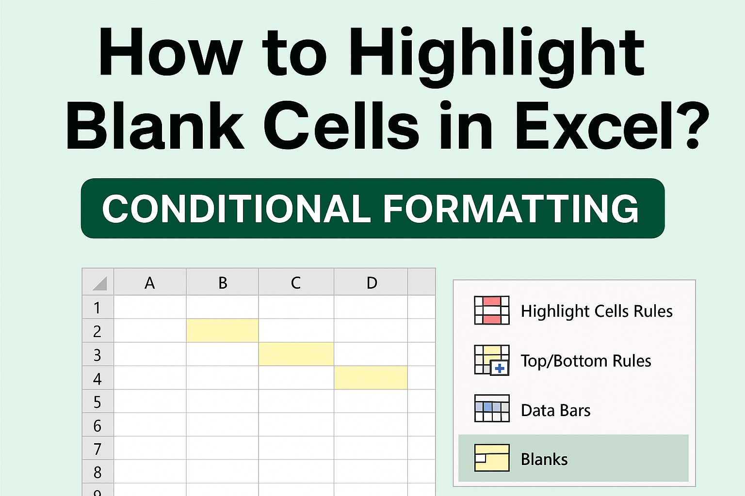
- Go to Home → Conditional Formatting → New Rule…
- Choose “Format only cells that contain”.
- In the rule dropdown, select Blanks.
- Click Format…, then choose a fill color (e.g. yellow) or any formatting you like — this will be applied to blank cells.
- Click OK → OK to apply. Now, all truly blank cells in the selected range are highlighted.
This method is quick, doesn’t need formulas, and works well when you just want obvious empty cells flagged.
Method 2: Use a Custom Formula (ISBLANK) for More Precision
If you want more control — or if some “empty-looking” cells contain formulas returning empty strings — use a formula-based rule:
- Select your range (for example B3:E20).
- Go to Home → Conditional Formatting → New Rule → Use a formula to determine which cells to format.
- Enter the formula (assuming your active cell is B3):
=ISBLANK(B3)This will mark cells that are truly empty. - Choose a format (fill color, border, font style) via Format…, then click OK → OK to apply.
⚠️ Note: The ISBLANK function only returns TRUE for truly empty cells (cells with absolutely nothing). It won’t catch cells that contain an empty string from a formula (""), or a space character.
Method 3: Highlight Cells That Appear Blank (Including Empty Strings / Formulas Returning “”)
If your worksheet may include cells that look blank but technically contain empty strings, you might prefer a more inclusive check. You can use a formula like:
=LEN(A2)=0
or
=A2=""
instead of ISBLANK. These treat empty-string cells as blank.
Steps:
- Select range → Conditional Formatting → New Rule → Use formula.
- Paste the formula (
=LEN(A2)=0, assuming A2 is top-left). - Format as desired → OK.
This catches more “blank-like” cells — helpful if cells contain formulas or invisible characters.
🧑💻 Final Thoughts
Highlighting blank cells with Conditional Formatting is a simple yet powerful way to catch missing data quickly — whether you’re preparing reports, cleaning datasets, or ensuring complete entries before analysis.
Once you set up a rule, the highlighting updates dynamically — meaning if someone fills in a cell later, the highlight goes away automatically. That’s much more efficient and safer than manual highlighting.