Freezing multiple rows and columns in Excel helps you keep important headers or labels visible while you scroll through large tables. This makes it easier to understand and compare data without losing track of what each row or column represents. In this blog, you will learn simple step-by-step instructions to freeze both rows and columns together using Excel’s Freeze Panes feature for a better working experience.
🛠️ Step-by-Step: How to Freeze Multiple Rows and/or Columns
Here’s a simple guide for freezing rows, columns, or a combination of both:
- Open your Excel worksheet where you want to freeze panes.
- Decide which rows and/or columns you want to freeze.
- To freeze multiple rows: choose the row just below the last row you want frozen.
- To freeze multiple columns: choose the column just to the right of the last column you want frozen.
- To freeze both rows and columns: click the cell that is immediately below the rows to freeze and immediately to the right of the columns to freeze.
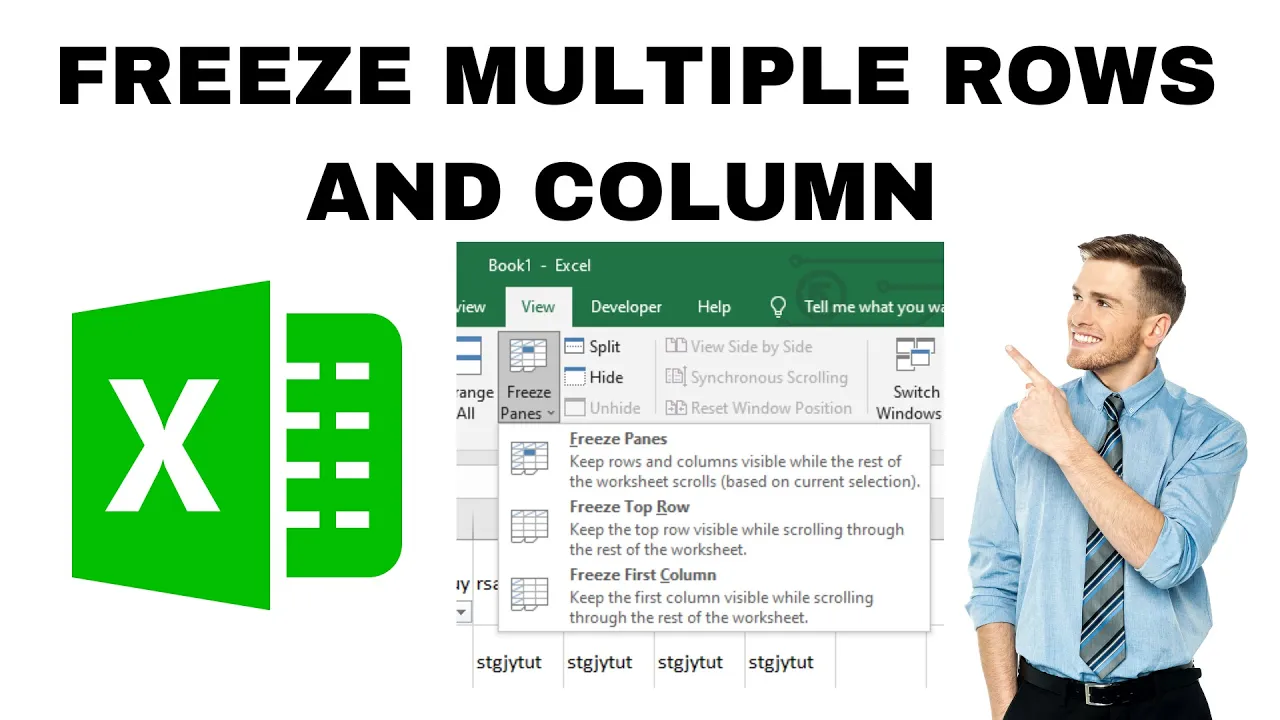
- Go to the “View” tab on the Excel ribbon.
- Click “Freeze Panes” (in the Window group), then select “Freeze Panes” from the dropdown.
- Verify: when you scroll, the rows and/or columns you froze should remain visible, while the rest of the sheet moves. Excel will draw subtle lines (horizontal and/or vertical) indicating where the freeze begins.