Finding duplicates in Excel is a quick way to clean up your data and avoid mistakes. Whether you’re working on a list of names, product codes, or numbers, duplicate entries can cause confusion and lead to errors in reports or calculations. Instead of checking each row manually, Excel gives you easy tools to spot and remove duplicates in just a few clicks. In this beginner-friendly blog, we’ll explain how to find duplicates in Excel step by step, so you can keep your spreadsheets neat and accurate.
Step-by-Step: How to Find Duplicates in Excel
Below are the simple steps to identify duplicate values in your worksheet.
✔ Step 1: Select the Data Range
First, highlight the cells you want to check for duplicates.
You can select:
- A single column
- Multiple columns
- An entire table
Make sure you select only the area where duplicates may exist.
✔ Step 2: Open Conditional Formatting
- Go to the Home tab
- Click Conditional Formatting
- Select Highlight Cells Rules
- Click Duplicate Values…
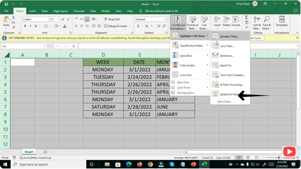
This opens the duplicate formatting dialog box.
✔ Step 3: Choose Formatting for Duplicates
In the popup window:
- From the dropdown, choose Duplicate
- Select a color—Excel highlights duplicates using formats like
- Light Red Fill
- Yellow Fill
- Green Text
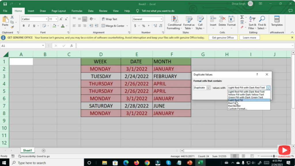
(You can pick any style depending on your preference.)
Click OK.
✔ Step 4: Duplicate Values Are Highlighted
Excel instantly highlights all duplicate cells in the selected range.
Now you can easily:
- Review duplicates
- Delete unnecessary entries
- Fix repeated data
This saves time and ensures clean, accurate spreadsheets.
Conclusion
Finding duplicates in Excel is quick and easy using Conditional Formatting. Whether you’re cleaning customer data, sales lists, or student records, Excel helps you identify repeat entries instantly. Following this step-by-step guide will help you maintain accuracy and reliability in your spreadsheets.