How to Compare Two Columns in Excel to Find Differences or Similarities

Comparing two columns in Excel is a powerful way to quickly spot differences or similarities in your data. Whether you’re working with lists of names, product IDs, or numbers, manually checking each entry can be time-consuming and prone to errors. Luckily, Excel provides built-in tools and formulas that make this process simple and efficient. In this beginner-friendly blog, we’ll explain in clear, step-by-step language how to compare two columns in Excel to find differences or similarities, so you can keep your spreadsheets accurate and organized.

---

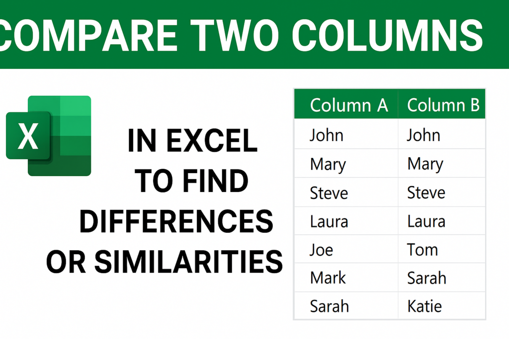
1. Compare Two Columns Using Conditional Formatting (Highlight Differences)

This method instantly highlights differences between Column A and Column B.

Steps:

1. Select the data in Column A.
2. Go to Home > Conditional Formatting > New Rule.
3. Choose “Use a formula to determine which cells to format.”
4. Enter the formula: =A1<>B1
5. Click Format, choose a highlight color, and press OK.

All values that do not match between the two columns will be highlighted.

---

2. Highlight Matching Values Between Two Columns

If you want to see which values are the same:

Steps:

1. Select Column A.
2. Go to Conditional Formatting > New Rule.
3. Use this formula: =A1=B1
4. Choose a highlight style and click OK.

Matching items will now be highlighted.

---

3. Compare Columns Using the IF Function

The IF formula helps you display whether values match or not.

Steps:

1. In a new column (Column C), enter: =IF(A1=B1, "Match", "Different")
2. Press Enter and drag the formula down.

Column C will clearly show “Match” or “Different” for each row.

---

4. Find Items in Column A That Are Not in Column B

Use the COUNTIF function to identify missing values.

Steps:

1. In Column C, enter: =IF(COUNTIF(B:B, A1)=0, "Not Found", "Found")
2. Copy the formula down.

This helps you find unique values in Column A that don’t exist in Column B.

---

5. Find Exact Differences Using the “Go To Special” Tool

This method highlights only the differences in selected ranges.

Steps:

1. Select Column A and Column B together.
2. Go to Home > Find & Select > Go To Special.
3. Choose Row differences.
4. Excel will highlight the mismatched cells.

---

6. Compare Tables Using VLOOKUP (For Larger Data Sets)

If the lists are in different locations or sheets:

Steps:

1. Use the formula: =IF(ISNA(VLOOKUP(A1, B:B, 1, FALSE)), "Not in B", "Match")
2. Drag it down.

This is helpful when comparing long lists.

---

Final Thoughts

Excel provides many ways to compare two columns — highlighted differences, formulas, and lookup functions. Choose the method that best fits your data. Using these steps, you can easily find similarities, mismatches, or missing items across any two columns.