Do you want your Excel sheet to be easier to read and more organized? One handy trick is to auto highlight the entire row when you select a cell. This makes it super simple to track data across columns without losing your place. Whether you’re working with big tables, reports, or lists, auto-highlighting rows can save time and reduce mistakes. In this blog, we’ll show you step-by-step how to set up automatic row highlighting in Excel, so your spreadsheets look cleaner and are easier to work with.

Step-by-Step: Set up Auto Highlight Row
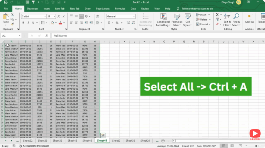
Step 1: Select the full sheet or area
- Click on the top-left corner between row numbers and column letters (or press Ctrl + A) to select the entire worksheet (or select the specific range where you want the effect).
Step 2: Open Conditional Formatting
- Go to the Home tab → click on Conditional Formatting → choose New Rule….
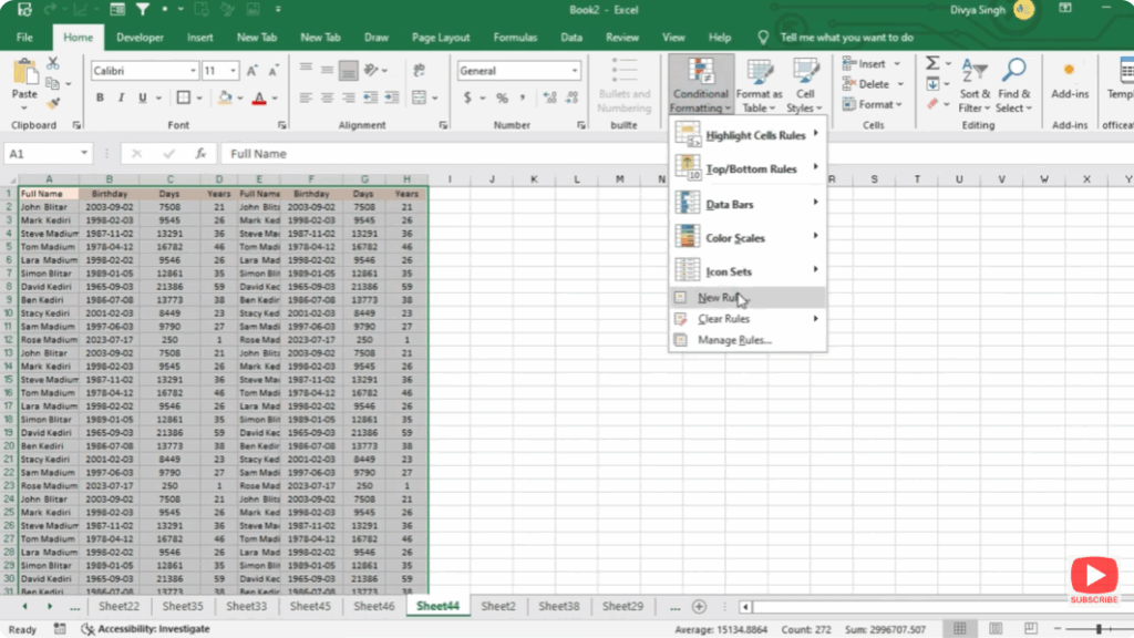
Step 3: Use a formula to determine which cells to format
- In the New Rule dialog, choose “Use a formula to determine which cells to format”.
- In the formula box, enter:
=ROW()=CELL("row",INDIRECT("RC",FALSE))or an alternative often-used formula:=ROW()=ROW(INDIRECT("RC",FALSE))(The exact structure may vary depending on how your version of Excel handles the INDIRECT/RC references.)
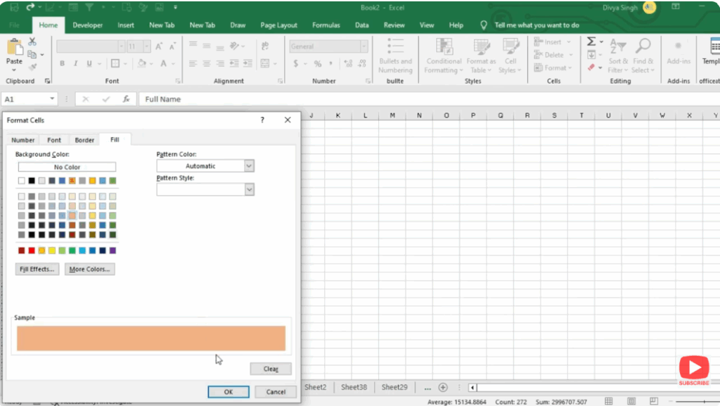
Step 4: Set the format
- Click Format…, go to Fill tab, choose a highlight colour (for example light yellow or grey).
- Click OK to apply the format.
Step 5: Confirm and test
- Click OK to close the New Rule dialog.
- Click any cell in your sheet — the entire row should now highlight automatically.
- Test by clicking on different rows; the formatting will shift to match the active row.
Final Thoughts
Setting up auto-highlight for the active row is a simple but effective way to improve readability, reduce errors, and enhance navigation in Excel. Once configured, your focus is clearer and your data interactions smoother.