
Navigating large Excel sheets can get confusing—especially when you lose track of which row you’re on. That’s where highlighting the active row becomes super helpful. Whenever you click on a cell, the entire row lights up, making it easier to read across columns.
You can achieve this using conditional formatting (no code needed) or via VBA for more dynamic behavior. Below are step-by-step methods.
✅ Method 1: Conditional Formatting (Formula-Based)
This is the easiest method and works in most Excel versions.
Steps
- Select the full rows / range where you want highlighting to apply
- For example, if your data is in rows 2 to 100, select the entire range A2:Z100 (or the full sheet).
- You can also select entire rows by clicking the row headers, but it’s safer to pick the columns you’ll use.
- Open Conditional Formatting
- Go to Home → Conditional Formatting → New Rule.
- Choose Use a formula to determine which cells to format.
- Enter the highlight formula
- In the formula box, type:
=ROW() = CELL("row") - This formula dynamically checks whether the row number for each cell’s row (
ROW()) matches the current active row (viaCELL("row")).
- In the formula box, type:
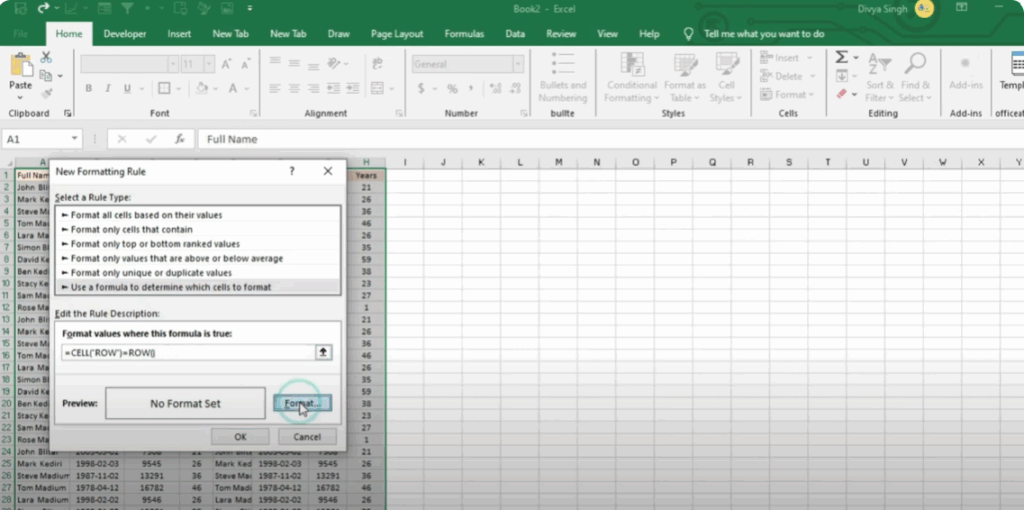
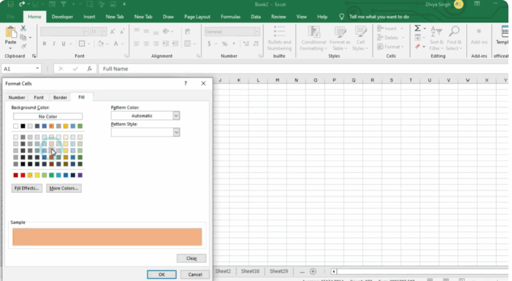
- Set the format (highlight style)
- Click Format… and choose a fill color (like light gray or another subtle shade), maybe bold font, etc.
- Click OK to confirm.
- Apply and test
- Click OK to finish the rule creation.
- Now, whenever you click any cell inside that range, the row should highlight.
✅ Final Thoughts
Automatically highlighting the active row can boost readability, reduce errors, and help you stay oriented in big spreadsheets. For most users, the conditional formatting formula approach is sufficient and easy to maintain. If you want your spreadsheet to feel more “alive,” the VBA solution gives you real-time responsiveness.