
Calculating discount percentages in Excel is simple and helps you quickly figure out savings on prices for sales, shopping lists, or business reports. Using basic formulas like (Original Price – Discounted Price) / Original Price * 100%, you can automate discount calculations across entire columns. In this blog, you’ll learn easy step-by-step methods to set up discount percentage formulas, format results as percentages, and create dynamic tables that update automatically when prices change.
How to Calculate Discount Percentages in Excel (Step-by-Step)
Step 1: Enter Your Data
Create a simple table with the following columns:
- Original Price
- Discounted Price
Example:
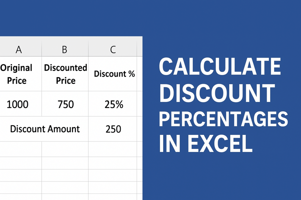
A2 = 1000
B2 = 750
Step 2: Apply the Discount Percentage Formula
To calculate the discount percentage, use this formula:
Formula:
=(A2 - B2) / A2
Here’s what it does:
- A2 = Original Price
- B2 = Discounted Price
- (A2 – B2) = Discount Amount
- Divide by A2 to convert it into a percentage
Step 3: Convert to Percentage Format
After applying the formula:
- Select the cell with the result
- Click on the Percent (%) button on the Home tab
- Increase decimal places if needed
You will now see something like:
25% discount
Step 4: Calculate Discount Amount (Optional)
If you want the price difference, use:
=A2 - B2
Example:
1000 – 750 = 250 discount
Step 5: Apply the Formula to Multiple Rows
Simply drag the fill handle (small square at bottom-right of the cell) down to apply the formula to all rows.
Conclusion
Calculating discount percentages in Excel only requires a simple formula. Whether you’re analyzing product prices, preparing invoices, or working in retail data, this technique saves time and reduces manual calculations. With just a few steps, Excel can give you accurate discount values instantly.