How to Create a Drop-Down list in Excel? Excel Cell

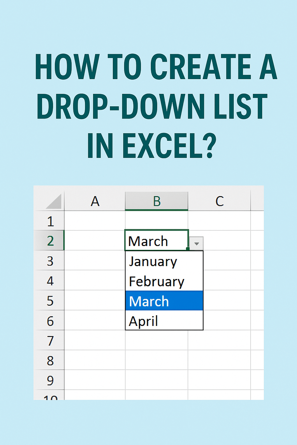
Creating a drop-down list in Excel is a simple way to make your spreadsheet more organized and easy to use. Instead of typing data manually every time, you can just pick an option from a ready-made list inside a cell. This helps avoid mistakes and saves time, especially when working with large sheets. The good news is, Excel has a built-in feature to create drop-down lists quickly. In this blog, we’ll explain step by step how to add a drop-down list in an Excel cell, using easy language so anyone can follow along.

---

🛠 Step-by-Step: Making a Drop-Down List

Here’s a clear guide to setting up a drop-down in a cell:

• Prepare the List Items
  • First, create your list of options in a column or row in Excel.
  • Alternatively, you can skip this and type your list items directly into the setup window later.
• Select the Cell for the Drop-Down
  • Click the cell (or cells) where you want the drop-down arrow to appear.
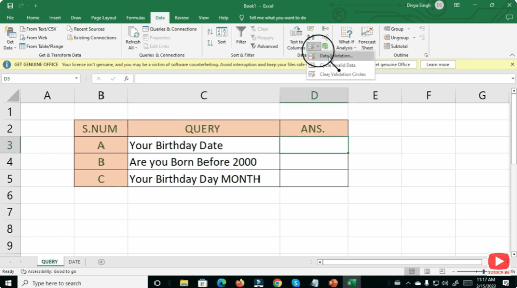
• Open Data Validation
  • Go to the Data tab on the ribbon.
  • In the Data Tools section, click Data Validation.

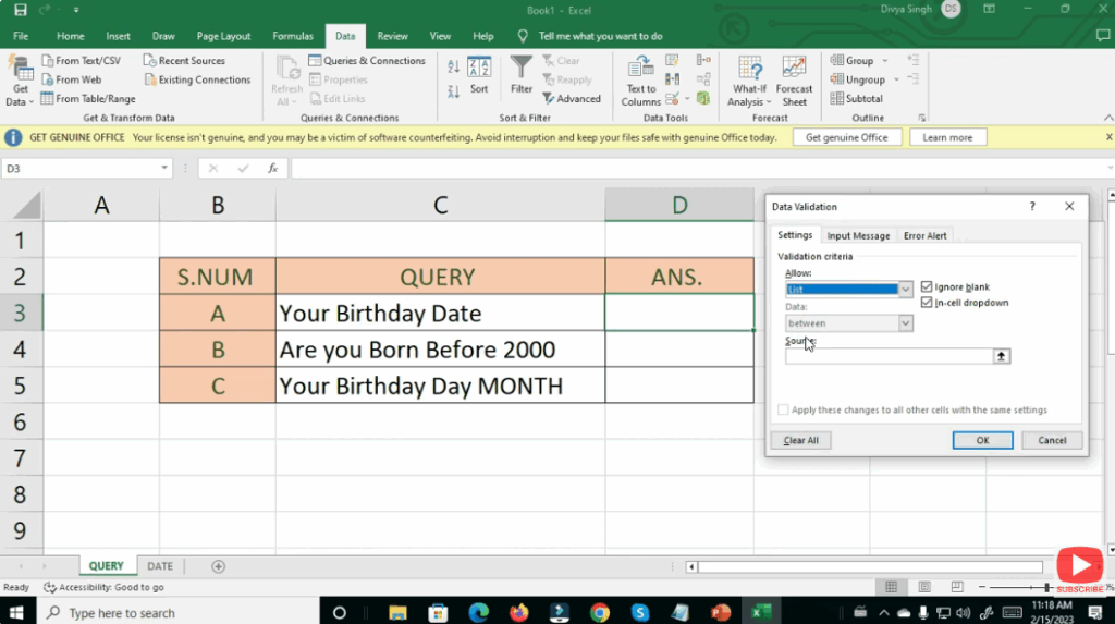
• Set Up the Validation Criteria
  • In the Data Validation dialog, go to the Settings tab.
  • In the Allow dropdown, select List.
  • In the Source field, either:
    • Type =A1:A5 (or wherever your list is).
    • Or, if manually entering: type Yes,No,Maybe separated by commas.
  • Make sure the checkbox In-cell dropdown is checked so the arrow appears next to the cell.

• Optional: Add Input Message
  • Switch to the Input Message tab.
  • Enable Show input message when cell is selected, then type a title and message (max ~225 characters).
  • This message appears when the user clicks the drop-down cell — great for instructions or guidance.
• Optional: Set an Error Alert
  • Go to the Error Alert tab.
  • Enable Show error alert after invalid data is entered.
  • Choose a style (Stop / Warning / Information) and write a message.
    • “Stop” prevents other entries.
    • “Warning” or “Information” lets people enter custom values.
• Click OK
  • After setting up, click OK to apply the validation.
  • You should now see a small arrow in the cell — click it to choose from your list.

---

✅ Final Thoughts

Creating a drop-down list in Excel is a great way to improve your data entry process. It ensures consistency, reduces typos, and speeds up input. Using Data Validation with lists — whether from an existing range or custom entries — gives you powerful control over your workbook.

Try it out in your next spreadsheet — and once you get comfortable, you can explore more advanced tricks like dynamic lists or dependent drop-downs. Happy spreadsheet building!