How to Create Filter in Excel

Creating a filter in Excel helps you quickly find and display only the data you need from large tables or lists. Filters add drop-down arrows to your column headers, letting you sort or show specific values, dates, or text easily without deleting or moving any data. This blog will guide you step-by-step on how to create and use filters in Excel to organize and analyze your data more effectively, even if you are a beginner.

---

Step-by-Step: How to Create a Filter in Excel

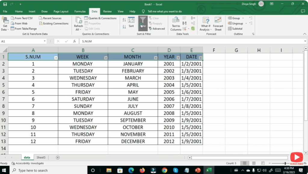
1. Enable the Filter Option

1. Open your Excel workbook and navigate to the worksheet you want to filter.
2. Select any cell in the data range (preferably within the headers of your table).
3. Go to the Data tab on the Ribbon → Click Filter.
4. You should now see small drop-down arrows next to each header cell.

---

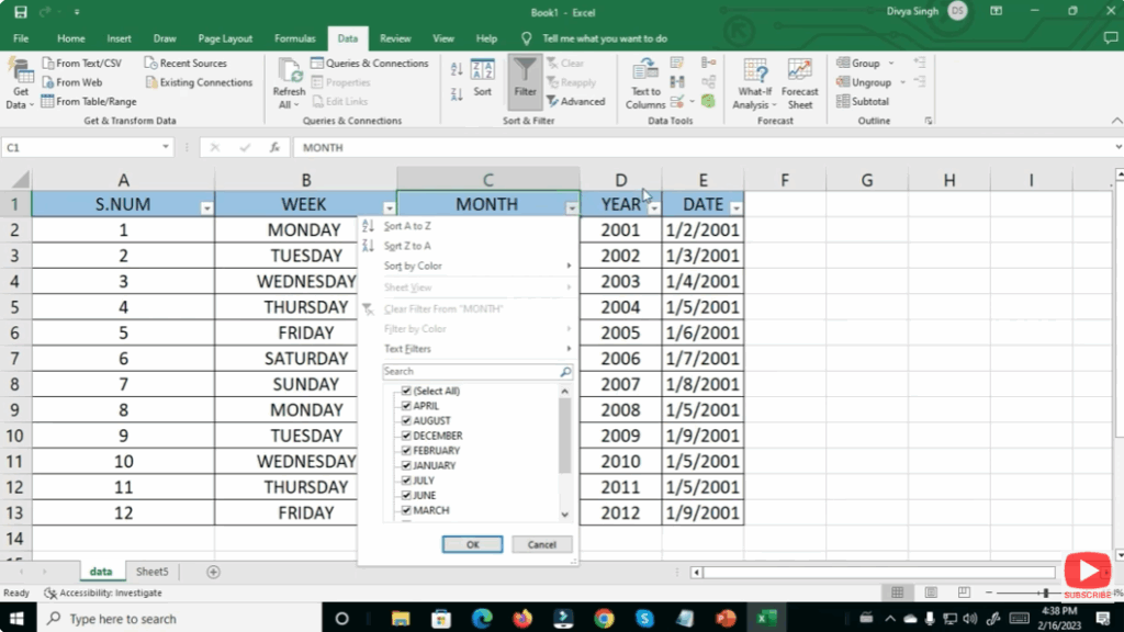
2. Apply a Basic Filter

1. Click the drop-down arrow on the column you want to filter.
2. In the filter menu, you can:
   • Search for specific values (if you have many distinct items)
   • Check / uncheck boxes for values you want to display or hide.
3. Click OK → Excel will hide all rows that do not match the selected criteria.

---

3. Use Text or Number Filters (Custom Criteria)

If you need more specific filtering (for example, “contains text” or “greater than a number”):

1. Open the filter drop-down arrow → go to Text Filters (for text) or Number Filters (for numbers).
2. Choose a condition (Equals, Contains, Greater Than, Between, etc.).
3. Enter your criteria in the dialog box → click OK. Excel will filter rows based on that condition.

---

Conclusion

Filters in Excel are fundamental for working efficiently with data. Whether you’re using the basic AutoFilter, advanced filtering, or dynamic array formulas like the FILTER function, Excel gives you flexible ways to view exactly the data you need. Mastering filters will make your spreadsheets far more powerful and user-friendly.