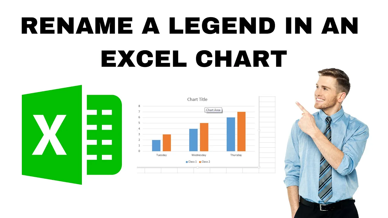
Want to make your Excel chart look clearer and more professional? Renaming the legend is a great way to help others understand your data better. The legend shows what each part of the chart represents, and sometimes the default names just aren’t helpful. Luckily, Excel gives you a couple of easy ways to change legend names to something more meaningful. In this blog, we’ll show you 2 simple methods to rename a legend in an Excel chart, step by step. Let’s make your charts easier to read and more polished!

🛠 Method 1: Change the Data Source Series Name Directly
This is generally the cleaner method.
- Select the chart containing the legend you want to change.
- Right-click one of the legend entries (or right-click the chart and choose Select Data).
- In the Select Data Source dialog, under Legend Entries (Series) you will see your series listed.
- Select the series whose legend you want to rename, and click Edit.
- In the Edit Series dialog, change the Series name field. You can:
- Type in a custom name directly (e.g.
"Sales 2025") - Or click the small box icon and pick a cell from your sheet that contains the desired name
- Type in a custom name directly (e.g.
- Click OK to close dialogs, and the legend in your chart will reflect the new name.
This method ensures the legend is dynamically tied to your worksheet data or your custom label.
🔧 Method 2: Edit the Legend Text in the Chart Itself (Quick Trick)
The video also shows a quicker, albeit more manual, way:
- Click the legend in your chart so that the legend entries become selectable.
- Then click the specific legend text you want to change — it goes into an edit mode (text box) for that legend entry.
- Type in your new legend text directly manually (for example, change “Series1” to “Projected Sales”).
- Press Enter or click away, and the legend updates to show your custom text.
Note: This method is more immediate and visual, but the legend text is no longer tied to your data — so if your data’s name changes, this manual label won’t automatically update.